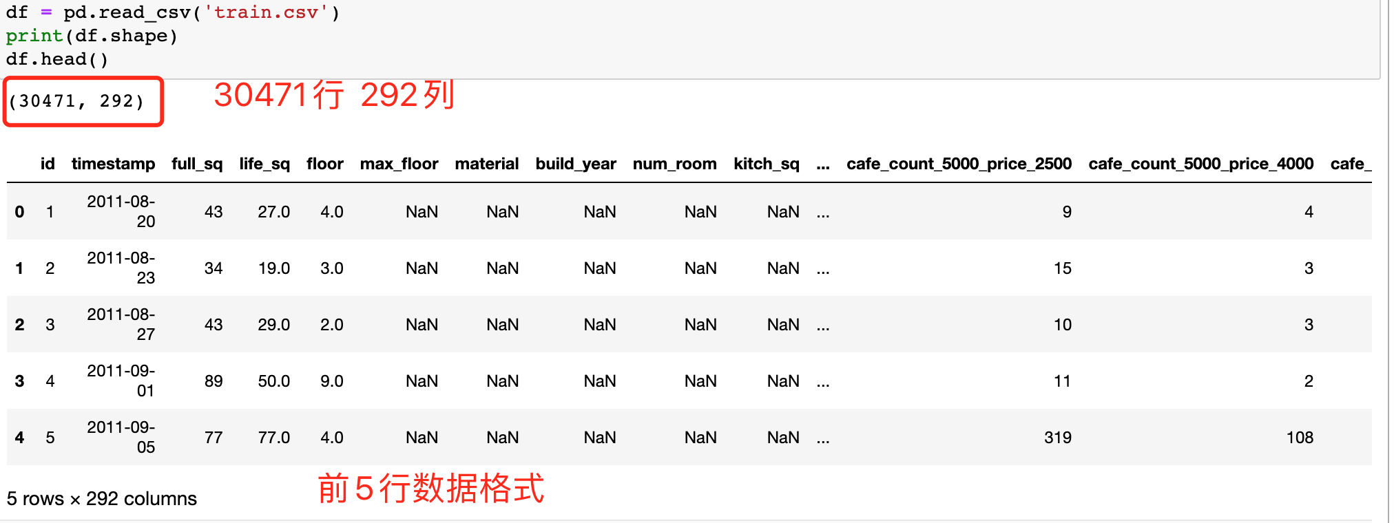
笔记数据集采用Kaggle竞赛Sberbank俄罗斯房地产价值预测竞赛数据 ,预测Russian房价波动。选取部分样本使用。数据集已统一放入Github中方便下载使用。train.csv ,数据集共有30471行、292列。
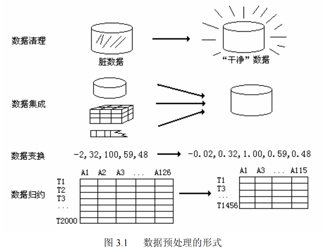
数据预处理的目的
去除不必要数据(重复、错误数据);不一致数据(大写、地址);不规则数据(异常值、脏数据)
补齐缺失值
对数据范围、量纲、格式、类型进行统一化处理,方便进行后续计算
数据集分析 1 2 3 4 5 6 7 import matplotlibimport matplotlib.pyplot as pltimport matplotlib.mlab as mlabfrom matplotlib.pyplot import figureimport numpy as npimport pandas as pdimport seaborn as sns
查看数据集基本信息 1 2 3 df = pd.read_csv('train.csv' ) print (df.shape)df.head()
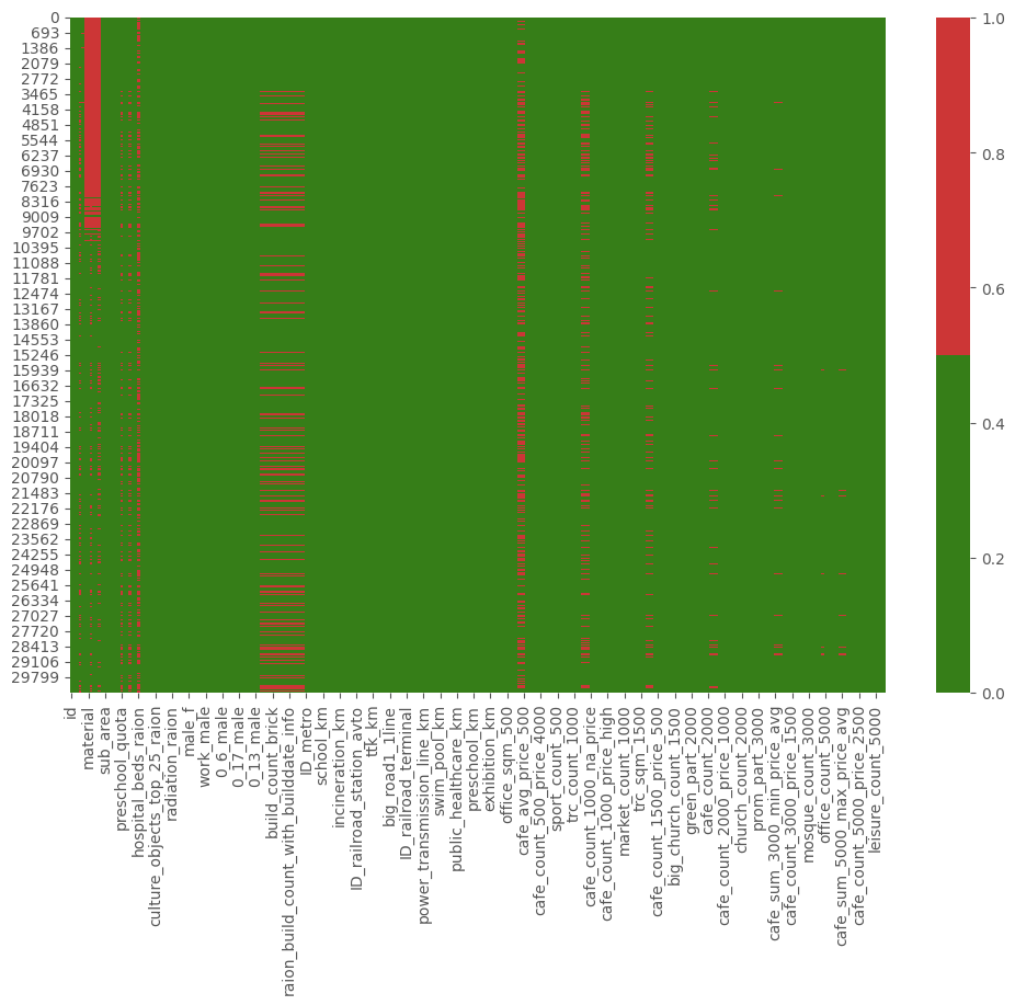
分析数据集缺失数据 热图缺失值分析 展示所有特征(所有列)的缺失数据,横轴代表特征名称,纵轴代表观察值,红色代表缺失数据 ,绿色代表非缺失数据 。
1 2 3 cols = df.columns[:df.shape[1 ]] colours = ['#367E18' , '#CC3636' ] sns.heatmap(df[cols].isnull(), cmap=sns.color_palette(colours))
注:图片颜色搭配使用Color Hunt
通过该缺失值热图,可以观察到在第0行至第7623行 的material 特征上全部缺失。第30000行后不缺失,可验证结果。
1 2 print (df.iloc[693 ]['material' ]) print (df.iloc[30000 ]['material' ])
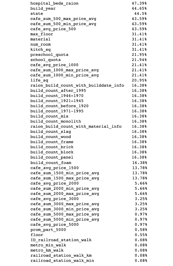
百分比缺失值分析 在热图的基础上,可通过对缺失值百分比列表来总结每个特征的的缺失百分比情况。
1 2 3 4 5 6 7 8 s = pd.Series(dtype=float ) for col in df.columns: pct_missing = np.mean(df[col].isnull()) if pct_missing > 0 : s[col] = round (pct_missing*100 , 2 ) print (s.sort_values(ascending=False ).to_string(float_format=lambda e:str (e)+'%' ))
可根据特征缺失百分比,选择要数据清理的特征。
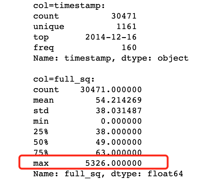
分析数据集不规则数据 百分比缺失值分析 1 2 3 4 5 6 7 8 9 10 index = 1 for col in df.columns: if index > 2 : break if col == 'id' : continue print ("col=%s:" %col) print (df[col].describe(), "\n" ) index+=1
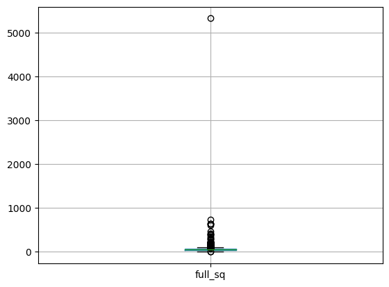
取了两列(timestamp和full_sq特征)的描述统计数据,可以看到full_sq在各分位数据的占比,以及最大、最小值。通过观察,最大值为5326,而在四分位(75个百分位)数据为63,因此最大值5326为异常值。
箱型图缺失值分析 1 2 df.boxplot(column=['full_sq' ])
通过箱型图可以观察到最高位置点5326为异常值,其他均小于1000。
其他查找异常值的方法还有散点图、z-score和聚类等,视情况选择。
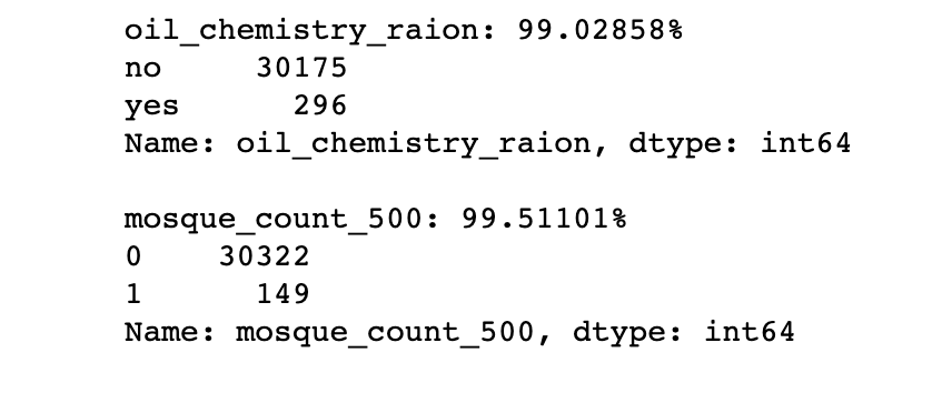
分析数据集不必要数据 百分比缺失值分析 1 2 3 4 5 6 7 8 9 10 11 num_rows = len (df.index) cols_percentage = [] for col in df.columns: cnts = df[col].value_counts(dropna=False ) top_pct = (cnts / num_rows).iloc[0 ] if top_pct > 0.99 : cols_percentage.append(col) print ('{0}: {1:.5f}%' .format (col, top_pct * 100 )) print (cnts) print ()
上图展示了99%的行是相同值的特征,所以需要逐一查看这些变量,了解背后的原因,以确认这些特征是否提供有用信息,如果无法提供有用信息,便可丢弃该特征。
重复行数据、关键特征重复行数据分析 1 2 3 4 5 6 7 8 9 10 11 12 13 df_dedupped = df.drop('id' , axis=1 ).drop_duplicates() print (df.shape)print (df_dedupped.shape)''' (30471, 292) (30461, 291) '''
可以看到除了id该列外(id自增,要先剔除掉),有10行数据为重复的,可以直接删除。
另外,还可以选中一组特征作为唯一标识符,然后基于这些特征检查是否存在复制数据。
分析数据集不一致数据 比如地名大小写不一致,应该全部转换为小写;时间格式不一致,可以统一转换为时间戳等;地址数据格式不一致等。
数据预处理方法 参考《数据挖掘概念与技术:韩家炜》第三章数据预处理。
数据清理 缺失值处理
删除变量/特征:缺失率较高(80%以上),且重要性较低,可以直接将变量/特征删除。(删除行或列)
统计量填充:缺失率较低(小于95%),且重要性较低,可根据数据分布,采用中位数进行填补。
插值法填充:随机插值、多重插补法、拉格朗日插值、牛顿插值。
模型填充:回归、贝叶斯、随机森林、决策树等对缺失值进行预测。
哑变量填充:变量为离散且不同值较少,可转换为哑变量。
离散点处理
要根据实际情况考虑离散点的数量和影响,是否需要。
数据集成 数据集成将多个数据源中的数据结合合成,存放在一个一致的数据仓库。不同的数据源,在合并时,保持规范化、去重。
数据变换(规范化处理) 1)标准化(均值移除) DeepLearning学习笔记-3-概率与信息论/#期望、方差和协方差 已总结过知识点。代码举例:
1 2 3 4 5 6 7 8 9 10 11 12 13 14 15 16 17 18 19 20 21 22 23 24 import numpy as npimport sklearn.preprocessing as spraw_samples = np.array([ [3.0 , -1.0 , 2.0 ], [0.0 , 4.0 , 3.0 ], [1.0 , -4.0 , 2.0 ] ]) print (raw_samples)print (raw_samples.mean(axis=0 )) print (raw_samples.std(axis=0 )) std_samples = raw_samples.copy() for col in std_samples.T: col_mean = col.mean() col_std = col.std() col -= col_mean col /= col_std print (std_samples)print (std_samples.mean(axis=0 ))print (std_samples.std(axis=0 ))
通过sklearn提供sp.scale函数实现同样的功能,代码所示:
1 2 3 4 std_samples = sp.scale(raw_samples) print (std_samples)print (std_samples.mean(axis=0 ))print (std_samples.std(axis=0 ))
2)范围缩放 将样本矩阵中的每一列最小值和最大值设定为相同的区间,统一各特征值的范围.如有a, b, c三个数,其中b为最小值,c为最大值,则:
$$
$$
缩放计算方式如下公式所示:
$$
$$
$$
计算完成后,最小值为0,最大值为1.以下是一个范围缩放的示例.
1 2 3 4 5 6 7 8 9 10 11 12 13 14 15 16 17 18 19 import numpy as npimport sklearn.preprocessing as spraw_samples = np.array([ [1.0 , 2.0 , 3.0 ], [4.0 , 5.0 , 6.0 ], [7.0 , 8.0 , 9.0 ]]).astype("float64" ) mms_samples = raw_samples.copy() for col in mms_samples.T: col_min = col.min () col_max = col.max () col -= col_min col /= (col_max - col_min) print (mms_samples)
我们也可以通过sklearn提供的对象实现同样的功能,如下面代码所示:
1 2 3 4 5 mms = sp.MinMaxScaler(feature_range=(0 , 1 )) mms_samples = mms.fit_transform(raw_samples) print (mms_samples)
执行结果:
1 2 3 4 5 6 [[0. 0. 0. ] [0.5 0.5 0.5] [1. 1. 1. ]] [[0. 0. 0. ] [0.5 0.5 0.5] [1. 1. 1. ]]
3)归一化 为了统一量纲,将所有的特征都统一到大致相同的数值范围内。常用方法:
Min-Max Scaling标准化:对原始数据进行线性变换,将结果映射到[0, 1]范围,实现对原始数据的等比缩放。
Z-Score Normalization标准化:将原始数据映射到均值为0、标准差为1的分布上,无量纲。
1 2 3 4 5 6 7 8 9 10 11 12 13 14 15 16 17 18 19 20 21 22 23 24 25 26 27 28 29 30 31 32 33 34 35 36 import numpy as npimport sklearn.preprocessing as spraw_samples = np.array([[1. , -1. , 2. ], [2. , 0. , 0. ], [0. , 1. , -1. ]]) min_max_samples = sp.MinMaxScaler().fit_transform(raw_samples) print (min_max_samples)""" [[0.5 0. 1. ] [1. 0.5 0.33333333] [0. 1. 0. ]] """ z_score_samples = sp.scale(raw_samples) print (z_score_samples)""" [[ 0. -1.22474487 1.33630621] [ 1.22474487 0. -0.26726124] [-1.22474487 1.22474487 -1.06904497]] """ print (z_score_samples.mean(axis=0 ))""" [0. 0. 0.] """ print (z_score_samples.std(axis=0 ))""" [1. 1. 1.] """
归一化适用的模型:通过梯度下降的模型通常需要归一化,包括线性模型、逻辑回归、支持向量机、神经网络等;决策树模型不适用归一化
4)二值化 根据一个事先给定的阈值,用0和1来表示特征值是否超过阈值.以下是实现二值化预处理的代码:
1 2 3 4 5 6 7 8 9 10 11 12 13 14 15 16 import numpy as npimport sklearn.preprocessing as spraw_samples = np.array([[65.5 , 89.0 , 73.0 ], [55.0 , 99.0 , 98.5 ], [45.0 , 22.5 , 60.0 ]]) bin_samples = raw_samples.copy() mask1 = bin_samples < 60 mask2 = bin_samples >= 60 bin_samples[mask1] = 0 bin_samples[mask2] = 1 print (bin_samples)
同样,也可以利用sklearn库来处理:
1 2 3 4 5 6 7 8 9 10 bin = sp.Binarizer(threshold=59 ) bin_samples = bin .transform(raw_samples) print (bin_samples)''' [[1. 1. 1.] [0. 1. 1.] [0. 0. 1.]] '''
二值化编码会导致信息损失,是不可逆的数值转换.如果进行可逆转换,则需要用到独热编码.
5)独热编码 DeepLearning学习笔记-6-深度前馈网络/#One-hot编码 已做过简单介绍。
$$\left[\begin{matrix}
对于第一列,有两个值,1使用10编码,7使用01编码
对于第二列,有三个值,3使用100编码,5使用010编码,8使用001编码
对于第三列,有四个值,2使用1000编码,4使用0100编码,6使用0010编码,9使用0001编码
编码字段,根据特征值的个数来进行编码,通过位置加以区分.通过独热编码后的结果为:
1 2 3 4 5 6 7 8 9 10 11 12 13 14 15 16 17 import numpy as npimport sklearn.preprocessing as spraw_samples = np.array([[1 , 3 , 2 ], [7 , 5 , 4 ], [1 , 8 , 6 ], [7 , 3 , 9 ]]) one_hot_encoder = sp.OneHotEncoder( sparse=False , dtype="int32" , categories="auto" ) oh_samples = one_hot_encoder.fit_transform(raw_samples) print (oh_samples)print (one_hot_encoder.inverse_transform(oh_samples))
执行结果:
1 2 3 4 5 6 7 8 9 [[1 0 1 0 0 1 0 0 0] [0 1 0 1 0 0 1 0 0] [1 0 0 0 1 0 0 1 0] [0 1 1 0 0 0 0 0 1]] [[1 3 2] [7 5 4] [1 8 6] [7 3 9]]
6)标签编码 根据字符串形式的特征值在特征序列中的位置,来为其指定一个数字标签,用于提供给基于数值算法的学习模型.代码如下所示:
1 2 3 4 5 6 7 8 9 10 11 12 import numpy as npimport sklearn.preprocessing as spraw_samples = np.array(['audi' , 'ford' , 'audi' , 'bmw' ,'ford' , 'bmw' ]) lb_encoder = sp.LabelEncoder() lb_samples = lb_encoder.fit_transform(raw_samples) print (lb_samples)print (lb_encoder.inverse_transform(lb_samples))
执行结果:
1 2 [0 2 0 1 2 1 ] ['audi ' 'ford ' 'audi ' 'bmw ' 'ford ' 'bmw ']
数据规约 维度规约 将不相关的特征、属性删除,减少数据量的同时要保证损失最小。
维度变换 降维,并且要保证数据的信息完整性。方法有主成分分析(PCA)和因子分析(FA);奇异值分解(SVD);聚类;流形学习等。
注意