Deeeplearning框架-PyTorch

PyTorch是一个建立在Torch库之上的Python包，是由Facebook开源的神经网络框架。它提供一种类似NumPy的抽象方法来表征张量（或多维数组），可利用GPU来加速训练。Torch是一个经典的对多维矩阵数据进行操作的张量（tensor ）库，包含自动求导系统的深度神经网络，提供了高度灵活性和效率的深度学习实验性平台。与Tensorflow的静态计算图不同，PyTorch的计算图是动态的，可以根据计算需要实时改变计算图。

安装

# CPU版本的
pip3 install torch torchvision torchaudio --index-url https://download.pytorch.org/whl/cpu
# CUDA 11.1
pip3 install torch torchvision torchaudio

PyTorch常用工具包

https://pytorch.org/docs/stable/torch.html

torch: 类似于Numpy的通用数组库，可将张量类型转为torch.cuda.TensorFloat，并在GPU上进行计算。
torch.autograd: 用于构建计算图形并自动获取梯度的包。
torch.nn: 具有共享层和损失函数的神经网络库。
torch.optim: 具有通用优化算法（如SGD，Adam等）的优化包。
torch.utils: 数据载入器。具有训练器和其他便利功能；

张量

张量形状术语

形状：张量的每个维度的长度（元素数量）。
秩：张量的维度数量。标量的秩为 0，向量的秩为 1，矩阵的秩为 2。
轴或维度：张量的一个特殊维度。
大小：张量的总项数，即乘积形状向量。

张量创建

method	desc
torch.tensor()	创建张量
torch.ones_like(x) torch.zeros_like(x) torch.rand_like(x)	创建一个与张量X具有相同维度的全1、全0或者是服从[0,1]区间上均匀分布的张量。
torch.normal(mean, std)	随机数生成张量，通过传入指定的均值张量和标准差张量，从而生成一个对应满足该分布的随机数张量。
torch.zeros(shape) torch.ones(shape) torch.eye(shape) torch.full(shape, fill_value) torch.empty(shape)	按照数值内容创建张量，可以通过指定shape来创建一个全0、全1、全为fill_value或是完全随机的一个张量。
torch.arange(start, end, step) torch.linspace(start, end, step) torch.logspace(start, end, step)	按照某种规则生成张量，可以通过指定start,end以及step参数来在某个范围内基于固定步长、等长间隔或对数间隔的张量。

与Numpy数据相互转化

method	desc
torch.as_tensor(ndarray) torch.from_numpy(ndarray)	将Numpy数组转化为PyTorch张量
tensor.numpy()	将PyTorch张量转化为Numpy数组

张量基本操作

索引与切片

遵循Python索引规则

索引从 0 开始编制
负索引表示按倒序编制索引
冒号 : 用于切片 start:stop:step

广播

广播是从 NumPy 中的等效功能借用的一个概念。简而言之，在一定条件下，对一组张量执行组合运算时，为了适应大张量，会对小张量进行“扩展”。
广播主要发生在两种情况，一种是两个张量的维数不相等，但是它们的后缘维度的轴长相符，另外一种是有一方的长度为1。

数学运算

自动求导

autograd模块

autograd包为对tensor进行自动求导，为实现对tensor自动求导，需考虑如下事项：

创建叶子节点(leaf node)的tensor，使用requires_grad参数指定是否记录对其的操作，以便之后利用backward()方法进行梯度求解。requires_grad参数缺省值为False，如果要对其求导需设置为True。
可利用requires_grad_()方法修改tensor的requires_grad属性。可以调用.detach()或with torch.no_grad():将不再计算张量的梯度，跟踪张量的历史记录。这点在评估模型、测试模型阶段常常使用。
通过运算创建的tensor（即非叶子节点），会自动被赋于grad_fn属性。该属性表示梯度函数。叶子节点的grad_fn为None。
最后得到的tensor执行backward()函数，此时自动计算各变量的梯度，并将累加结果保存grad属性中。计算完成后，非叶子节点的梯度自动释放。
backward()函数接受参数，该参数应和调用backward()函数的Tensor的维度相同。如果求导的tensor为标量（即一个数字），backward中参数可省略。
反向传播的中间缓存会被清空，如果需要进行多次反向传播，需要指定backward中的参数retain_graph=True。多次反向传播时，梯度是累加的。
非叶子节点的梯度backward调用后即被清空。
可以通过用torch.no_grad()包裹代码块来阻止autograd去跟踪那些标记为.requesgrad=True的张量的历史记录。这步在测试阶段经常使用。
整个过程中，Pytorch采用计算图的形式进行组织，该计算图为动态图，它的计算图在每次前向传播时，将重新构建。其他深度学习架构，如TensorFlow、Keras一般为静态图。

标量反向传播

假设x、w、b都是标量，z=wx+b，对标量z调用backward()，无需对backward()传入参数。

1
2
3

z.backward()
print(w.grad)
print(b.grad)

非标量反向传播

Pytorch有个简单的规定，不让张量(tensor)对张量求导，只允许标量对张量求导，因此，如果目标张量对一个非标量调用backward()，需要传入一个gradient参数,该参数也是张量，而且需要与调用backward()的张量形状相同。

"""
 非标量反向传播
"""
import torch
# 定义叶子节点张量x,y
a = torch.tensor([2, 3], dtype=torch.float, requires_grad=True)
b = torch.tensor([5, 6], dtype=torch.float, requires_grad=True)
# 定义f与a,b之间的映射关系：
f = a * b
# 反向传播
# 这里f是非标量张量所以我们需要把梯度参数传递给和张量f维数相同的反向传播函数
gradients = torch.ones_like(f)
f.backward(gradient=gradients)

print(a.grad)   # tensor([5., 6.])
print(b.grad)   # tensor([2., 3.])

tensorflow的forward只会根据第一次模型前向传播来构建一个静态的计算图, 后面的梯度自动求导都是根据这个计算图来计算的, 但是pytorch则不是, 它会为每次forward计算都构建一个动态图的计算图, 后续的每一次迭代都是使用一个新的计算图进行计算的.非常灵活，易调节

数据加载

torch.utils.data.Dataset: 实现对数据的加载。
torch.utils.data.TensorDataset: 对tensor进行打包
torch.utils.data.DataLoader: 数据加载器，结合了数据集和取样器，并且可以提供多个线程处理数据集。

1	torch.utils.data.DataLoader(dataset, batch_size=1, shuffle=False, num_workers=0, drop_last=False)

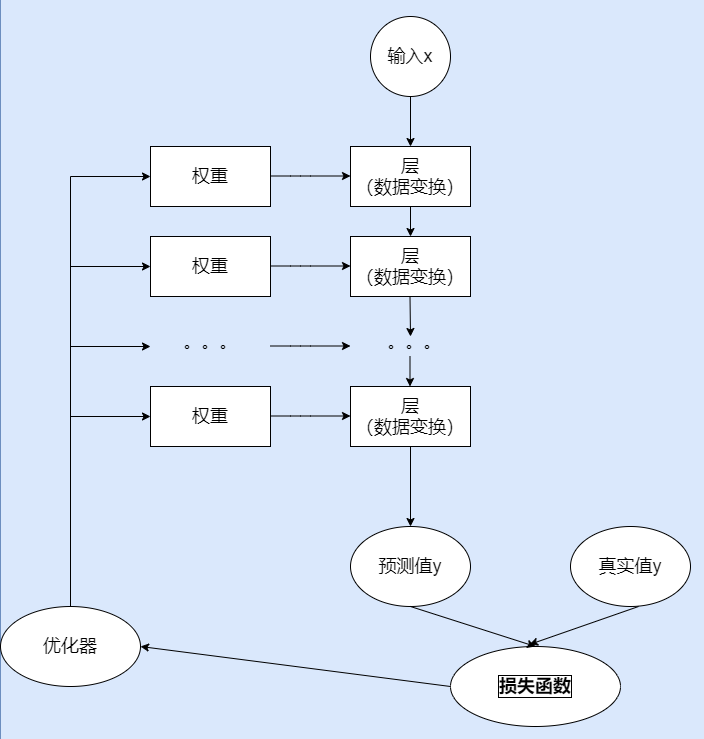
PyTorch神经网络

核心组件

层：神经网络的基本结构，将输入张量转换为输出张量。
模型：层构成的网络。
损失函数：参数学习的目标函数，通过最小化损失函数来学习各种参数。
优化器：如何使得损失函数最小，这就涉及到优化器。

PyTorch的nn模块

nn全称为neural network,意思是神经网络，是torch中构建神经网络的模块，导入为torch.nn。

[https://pytorch.org/docs/stable/nn.html][https://pytorch.org/docs/stable/nn.html]

常用卷积层

https://pytorch.org/docs/stable/nn.html#convolution-layers

1	torch.nn.Conv2d(in_channels, out_channels, kernel_size, stride=1, padding=0, dilation=1, groups=1, bias=True, padding_mode='zeros', device=None, dtype=None)

in_channels (int) – Number of channels in the input image
out_channels (int) – Number of channels produced by the convolution
kernel_size (int or tuple) – Size of the convolving kernel
stride (int or tuple, optional) – Stride of the convolution. Default: 1
padding (int, tuple or str, optional) – Padding added to all four sides of the input. Default: 0
padding_mode (str, optional) – ‘zeros’, ‘reflect’, ‘replicate’ or ‘circular’. Default: ‘zeros’
dilation (int or tuple, optional) – Spacing between kernel elements. Default: 1
groups (int, optional) – Number of blocked connections from input channels to output channels. Default: 1
bias (bool, optional) – If True, adds a learnable bias to the output. Default: True

常用池化层

https://pytorch.org/docs/stable/nn.html#pooling-layers

1	torch.nn.MaxPool2d(kernel_size, stride=None, padding=0, dilation=1, return_indices=False, ceil_mode=False)

kernel_size (Union[int, Tuple[int, int]]) – the size of the window to take a max over
stride (Union[int, Tuple[int, int]]) – the stride of the window. Default value is kernel_size
padding (Union[int, Tuple[int, int]]) – Implicit negative infinity padding to be added on both sides
dilation (Union[int, Tuple[int, int]]) – a parameter that controls the stride of elements in the window
return_indices (bool) – if True, will return the max indices along with the outputs. Useful for torch.nn.MaxUnpool2d later
ceil_mode (bool) – when True, will use ceil instead of floor to compute the output shape

激活函数

https://pytorch.org/docs/stable/nn.html#non-linear-activations-weighted-sum-nonlinearity

# https://pytorch.org/docs/stable/generated/torch.nn.ReLU.html#torch.nn.ReLU
torch.nn.ReLU()
# https://pytorch.org/docs/stable/generated/torch.nn.Sigmoid.html#torch.nn.Sigmoid
torch.nn.Sigmoid()
# https://pytorch.org/docs/stable/generated/torch.nn.Softmax.html#torch.nn.Softmax
torch.nn.Softmax()
# https://pytorch.org/docs/stable/generated/torch.nn.Tanh.html#torch.nn.Tanh
torch.nn.Tanh()

损失函数

https://pytorch.org/docs/stable/nn.html#loss-functions

# 创建一个衡量输入`x`(`模型预测输出`)和目标`y`之间均方误差标准。常用于回归模型。
torch.nn.MSELoss(size_average=True)
  
# 交叉熵损失函数，又称对数似然损失函数，常用于分类模型。
torch.nn.CrossEntropyLoss(weight=None, size_average=True)

全连接层

https://pytorch.org/docs/stable/nn.html#linear-layers

# 线性变换
"""
in_features - 每个输入样本的大小
out_features - 每个输出样本的大小
bias - 若设置为False，这层不会学习偏置。默认值：True
"""
torch.nn.Linear(in_features, out_features, bias=True)

防止过拟合函数

https://pytorch.org/docs/stable/nn.html#normalization-layers

"""
对小批量(mini-batch)数据进行批标准化(Batch Normalization)操作

num_features： 来自期望输入的特征数
eps： 为保证数值稳定性（分母不能趋近或取0）,给分母加上的值。默认为1e-5。
momentum： 动态均值和动态方差所使用的动量。默认为0.1。
affine： 一个布尔值，当设为true，给该层添加可学习的仿射变换参数。
"""
torch.nn.BatchNorm2d(num_features, eps=1e-05, momentum=0.1, affine=True)

# 随机将输入张量中部分元素设置为0。对于每次前向调用，被置0的元素都是随机的。
# p - 将元素置0的概率。默认值：0.5
torch.nn.Dropout(p=0.5)

其他

https://pytorch.org/docs/stable/nn.html#transformer-layers

构建神经网络容器

自定义神经网络。构建网络层可以基于Module类，即torch.nn.Module，它是所有网络的基类。

nn.Module与nn.functional的区别：
nn中的层，

一类是继承了nn.Module，其命名一般为nn.Xxx(第一个是大写),如nn.Linear、nn.Conv2d、nn.CrossEntropyLoss等。
另一类是nn.functional中的函数，其名称一般为nn.functional.xxx，如nn.functional.linear、nn.functional.conv2d、nn.functional.cross_entropy等。

从功能来说两者相当，基于nn.Mudle能实现的层，使用nn.functional也可实现，反之亦然，而且性能方面两者也没有太大差异。但PyTorch官方推荐：具有学习参数的（例如，conv2d, linear, batch_norm)采用nn.Xxx方式。没有学习参数的（例如，maxpool, loss func, activation func）等根据个人选择使用nn.functional.xxx或者nn.Xxx方式。

PyTorch优化器

torch.optim.SGD


"""
可实现SGD优化算法，带动量SGD优化算法，带NAG(Nesterov accelerated gradient)动量SGD优化算法,并且均可拥有weight_decay项。

params(iterable)- 参数组，优化器要管理的那部分参数。
lr(float)- 初始学习率，可按需随着训练过程不断调整学习率。
momentum(float)- 动量，通常设置为0.9，0.8
"""
torch.optim.SGD(params, lr, momentum=0)

torch.optim.Adam(AMSGrad)


"""
Adam(Adaptive Moment Estimation)本质上是带有动量项的RMSprop，它利用梯度的一阶矩估计和二阶矩估计动态调整每个参数的学习率。Adam的优点主要在于经过偏置校正后，每一次迭代学习率都有个确定范围，使得参数比较平稳。
"""
torch.optim.Adam(params, lr=0.001, betas=(0.9, 0.999), eps=1e-08)

torch.optim.Adagrad


"""
实现Adagrad优化方法(Adaptive Gradient)，Adagrad是一种自适应优化方法，是自适应的为各个参数分配不同的学习率。这个学习率的变化，会受到梯度的大小和迭代次数的影响。梯度越大，学习率越小；梯度越小，学习率越大。缺点是训练后期，学习率过小，因为Adagrad累加之前所有的梯度平方作为分母。AdaGrad算法是通过参数来调整合适的学习率λ，能独立地自动调整模型参数的学习率，对稀疏参数进行大幅更新和对频繁参数进行小幅更新。因此，Adagrad方法非常适合处理稀疏数据。AdaGrad算法在某些深度学习模型上效果不错。但还有些不足，可能因其累积梯度平方导致学习率过早或过量的减少所致。
"""
torch.optim.Adagrad(params, lr=0.01, lr_decay=0, weight_decay=0, initial_accumulator_value=0)

模型搭建步骤

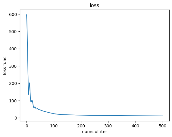
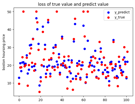
项目一：CNN回归模型之波士顿房价预测

# 导包
from sklearn.preprocessing import MinMaxScaler
from torch import nn
import matplotlib.pyplot as plt
import numpy as np
import pandas as pd
import torch
# 导入数据集
from sklearn.model_selection import train_test_split


# 数据加载
data_url = "http://lib.stat.cmu.edu/datasets/boston"
raw_df = pd.read_csv(data_url, sep="\s+", skiprows=22, header=None)
data = np.hstack([raw_df.values[::2, :], raw_df.values[1::2, :2]])
target = raw_df.values[1::2, 2]


X = data    # 特征提取
Y = target  # 目标target提取
Y = Y.reshape(-1, 1)    # 将y转换为一个列

# 数据归一化
ss = MinMaxScaler()
X = ss.fit_transform(X)

# 把x，y从ndarray格式转成tensor格式
X = torch.from_numpy(X).type(torch.FloatTensor)
Y = torch.from_numpy(Y).type(torch.FloatTensor)

# 切分数据集
train_x, test_x, train_y, test_y = train_test_split(X, Y, test_size=0.2)

# 构建网络
model = nn.Sequential(
    nn.Linear(13, 16), # 13*16 输入train_x的维度是(404,13)
    nn.ReLU(),  # ReLU()层  输出的数据的维度(404,16)
    nn.Linear(16, 1)   # 再加一层全连接层 就输出y了  维度是(404,1)
)

# 构建优化器和损失函数
criterion = nn.MSELoss()
optimizer = torch.optim.Adam(model.parameters(), lr=0.08)

# 训练
max_epoch = 500
iter_loss = []
for i in range(max_epoch):
    # 向前传播
    y_pred = model(train_x)
    # 计算loss
    loss = criterion(y_pred, train_y)
    if (i % 50 == 0):
        print("第{}次迭代的loss是:{}".format(i, loss))
    
    iter_loss.append(loss.item())
    # 清空之前的梯度
    optimizer.zero_grad()
    # 反向传播
    loss.backward()
    # 权重调整
    optimizer.step()

# 测试
output = model(test_x)
predict_list = output.detach().numpy()
print(predict_list[:10])    # 只输出10行

# 绘制不同的iteration的loss
x = np.arange(max_epoch)
y = np.array(iter_loss)
plt.figure()
plt.plot(x, y)
plt.title('loss')
plt.xlabel('nums of iter')
plt.ylabel('loss func')
plt.show()

# 查看真实值与预测值的散点图
x = np.arange(test_x.shape[0])
y1 = np.array(predict_list) # 测试集的预测值
y2 = np.array(test_y) # 测试集的实际值
line1 = plt.scatter(x, y1, c='blue')
line2 = plt.scatter(x, y2, c='red')
plt.legend([line1, line2], ['y_predict', 'y_true'])
plt.title("loss of true value and predict value")
plt.ylabel('boston hoursing price')
plt.show()

outputs:

第0次迭代的loss是:596.5716552734375
第50次迭代的loss是:46.23166275024414
第100次迭代的loss是:24.163291931152344
第150次迭代的loss是:17.612567901611328
第200次迭代的loss是:15.434951782226562
第250次迭代的loss是:14.168197631835938
第300次迭代的loss是:13.293211936950684
第350次迭代的loss是:12.607232093811035
第400次迭代的loss是:12.067901611328125
第450次迭代的loss是:11.588809967041016
[[12.9814005]
 [21.10761  ]
 [16.77605  ]
 [21.558886 ]
 [21.683792 ]
 [20.60617  ]
 [20.92336  ]
 [25.620314 ]
 [15.320004 ]
 [17.533672 ]]

项目二：MNIST手写字体识别


import torch
import torch.nn as nn
import torchvision
import torch.nn.functional as F
import torch.utils.data as Data
from torch.autograd import Variable
import matplotlib.pyplot as plt


EPOCH = 3
BATCH_SIZE=50
LR = 0.001

root_dataset = './dataset'
train_data = torchvision.datasets.MNIST(
    root=root_dataset,
    train=True,
    transform=torchvision.transforms.ToTensor(),
    download=True
)

# 显式图片
# print(train_data.train_data.size())
# print(train_data.train_labels.size())

# plt.imshow(train_data.train_data[66].numpy(), cmap='Greys')
# plt.title("%i" % train_data.train_labels[66])
# plt.show()

# 加载训练数据
train_loader = Data.DataLoader(
    dataset=train_data,
    batch_size=BATCH_SIZE,
    shuffle=True
)

# 加载测试集数据
test_data = torchvision.datasets.MNIST(
    root=root_dataset,
    train=False,
    download=True
)

test_x = torch.unsqueeze(test_data.test_data, dim=1).type(torch.FloatTensor)[:2000]/255
test_y = test_data.test_labels[:2000]


class CNN(nn.Module):
    def __init__(self):
        super(CNN, self).__init__()
        self.conv1 = nn.Sequential(
            # 卷积 维度变换（1,28,28）--> (16,28,28)
            nn.Conv2d(in_channels=1,  # 输入信号通道
                     out_channels=16, # 输出信号通道
                     kernel_size=3,   # 卷积核尺寸
                     stride=1,        # 卷积步长
                     padding=1        # 每一条边补充0的层数
                     ),
            # 激活函数
            nn.ReLU(),
            # 最大池化
            nn.MaxPool2d(kernel_size=2) # 维度变换（16,28,28）--> (16,14,14)
        )
        
        self.conv2 = nn.Sequential(
            # 卷积 维度变换(16,14,14) --> (32,14,14)
            nn.Conv2d(in_channels=16,
                     out_channels=32,
                     kernel_size=3,
                     stride=1,
                     padding=1
                     ),
            # 激活函数
            nn.ReLU(),
            # 最大池化
            nn.MaxPool2d(kernel_size=2)  # 维度变换(32,14,14) --> (32,7,7)
        )
        
        # 全连接
        self.output = nn.Linear(32*7*7, 10)
        
    def forward(self, x):
        out = self.conv1(x)
        out = self.conv2(out)
        out = out.view(out.size(0), -1)
        out = self.output(out)
        
        return out


cnn = CNN()

# 定义优化器
optimizer = torch.optim.Adam(cnn.parameters(), lr=LR)

# 定义损失函数
loss_func = nn.CrossEntropyLoss()

# 开始训练
for epoch in range(EPOCH):
    for step, (b_x, b_y) in enumerate(train_loader):
        # 计算模型输出值
        output = cnn(b_x) 
        # 计算损失函数
        loss = loss_func(output, b_y)
        # 优化器清零
        optimizer.zero_grad()
        # loss反向传播
        loss.backward()
        # 优化器优化
        optimizer.step()
        
        if step % 50 == 0:
            test_output = cnn(test_x)
            pred_y = torch.max(test_output, 1)[1].data.numpy()
            accuracy = float((pred_y == test_y.data.numpy()).astype(int).sum()) / float(test_y.size(0))
            print('epoch: {} step: {} train loss: {} test accuracy: {}'.format(epoch, step, loss.data.numpy(), accuracy))
            

# 保存模型
torch.save(cnn, './checkpoint/cnn_minist.pkl')
print('training finished')

outputs:

epoch: 0 step: 0 train loss: 2.2989518642425537 test accuracy: 0.124
epoch: 0 step: 50 train loss: 0.6227200627326965 test accuracy: 0.761
epoch: 0 step: 100 train loss: 0.255100816488266 test accuracy: 0.873
epoch: 0 step: 150 train loss: 0.12506981194019318 test accuracy: 0.9035
epoch: 0 step: 200 train loss: 0.23605869710445404 test accuracy: 0.916
epoch: 0 step: 250 train loss: 0.10597402602434158 test accuracy: 0.9245
epoch: 0 step: 300 train loss: 0.19649431109428406 test accuracy: 0.9365
epoch: 0 step: 350 train loss: 0.09695011377334595 test accuracy: 0.945
epoch: 0 step: 400 train loss: 0.169553741812706 test accuracy: 0.9445
epoch: 0 step: 450 train loss: 0.07386567443609238 test accuracy: 0.956
epoch: 0 step: 500 train loss: 0.09177689254283905 test accuracy: 0.9525
epoch: 0 step: 550 train loss: 0.249346062541008 test accuracy: 0.957
epoch: 0 step: 600 train loss: 0.3329342305660248 test accuracy: 0.956
epoch: 0 step: 650 train loss: 0.2073971927165985 test accuracy: 0.9625
epoch: 0 step: 700 train loss: 0.07403621822595596 test accuracy: 0.964
epoch: 0 step: 750 train loss: 0.05281904339790344 test accuracy: 0.9615
epoch: 0 step: 800 train loss: 0.07417619973421097 test accuracy: 0.961
epoch: 0 step: 850 train loss: 0.1186814084649086 test accuracy: 0.9705
epoch: 0 step: 900 train loss: 0.11796750128269196 test accuracy: 0.965
epoch: 0 step: 950 train loss: 0.020582687109708786 test accuracy: 0.9715
epoch: 0 step: 1000 train loss: 0.028191855177283287 test accuracy: 0.9655
epoch: 0 step: 1050 train loss: 0.10790297389030457 test accuracy: 0.967
epoch: 0 step: 1100 train loss: 0.037335075438022614 test accuracy: 0.9635
epoch: 0 step: 1150 train loss: 0.1390017867088318 test accuracy: 0.9655
epoch: 1 step: 0 train loss: 0.07538899779319763 test accuracy: 0.9715
epoch: 1 step: 50 train loss: 0.06148580089211464 test accuracy: 0.9745
epoch: 1 step: 100 train loss: 0.059671998023986816 test accuracy: 0.9635
epoch: 1 step: 150 train loss: 0.0580081082880497 test accuracy: 0.9745
epoch: 1 step: 200 train loss: 0.012145531363785267 test accuracy: 0.97
epoch: 1 step: 250 train loss: 0.03478122875094414 test accuracy: 0.972
epoch: 1 step: 300 train loss: 0.03409402817487717 test accuracy: 0.9675
epoch: 1 step: 350 train loss: 0.03502879664301872 test accuracy: 0.9725
epoch: 1 step: 400 train loss: 0.03113013319671154 test accuracy: 0.978
epoch: 1 step: 450 train loss: 0.13314753770828247 test accuracy: 0.978
epoch: 1 step: 500 train loss: 0.018445264548063278 test accuracy: 0.97
epoch: 1 step: 550 train loss: 0.011954346671700478 test accuracy: 0.973
epoch: 1 step: 600 train loss: 0.0324656218290329 test accuracy: 0.9775
epoch: 1 step: 650 train loss: 0.046384457498788834 test accuracy: 0.9745
epoch: 1 step: 700 train loss: 0.05520062893629074 test accuracy: 0.979
epoch: 1 step: 750 train loss: 0.30722805857658386 test accuracy: 0.9765
epoch: 1 step: 800 train loss: 0.10514361411333084 test accuracy: 0.9765
epoch: 1 step: 850 train loss: 0.04414287954568863 test accuracy: 0.981
epoch: 1 step: 900 train loss: 0.1443830281496048 test accuracy: 0.978
epoch: 1 step: 950 train loss: 0.026100166141986847 test accuracy: 0.979
epoch: 1 step: 1000 train loss: 0.11013159900903702 test accuracy: 0.9795
epoch: 1 step: 1050 train loss: 0.10890169441699982 test accuracy: 0.977
epoch: 1 step: 1100 train loss: 0.07636130601167679 test accuracy: 0.98
epoch: 1 step: 1150 train loss: 0.12814483046531677 test accuracy: 0.9795
epoch: 2 step: 0 train loss: 0.15829549729824066 test accuracy: 0.977
epoch: 2 step: 50 train loss: 0.022714903578162193 test accuracy: 0.976
epoch: 2 step: 100 train loss: 0.11526823043823242 test accuracy: 0.98
epoch: 2 step: 150 train loss: 0.042159732431173325 test accuracy: 0.979
epoch: 2 step: 200 train loss: 0.10546272993087769 test accuracy: 0.979
epoch: 2 step: 250 train loss: 0.030654177069664 test accuracy: 0.98
epoch: 2 step: 300 train loss: 0.0656307265162468 test accuracy: 0.9795
epoch: 2 step: 350 train loss: 0.08443894982337952 test accuracy: 0.978
epoch: 2 step: 400 train loss: 0.035659801214933395 test accuracy: 0.976
epoch: 2 step: 450 train loss: 0.08835320174694061 test accuracy: 0.979
epoch: 2 step: 500 train loss: 0.02448669634759426 test accuracy: 0.976
epoch: 2 step: 550 train loss: 0.023640567436814308 test accuracy: 0.98
epoch: 2 step: 600 train loss: 0.0034627816639840603 test accuracy: 0.9775
epoch: 2 step: 650 train loss: 0.10121780633926392 test accuracy: 0.9785
epoch: 2 step: 700 train loss: 0.0032379289623349905 test accuracy: 0.9795
epoch: 2 step: 750 train loss: 0.053985223174095154 test accuracy: 0.9805
epoch: 2 step: 800 train loss: 0.014309514313936234 test accuracy: 0.9805
epoch: 2 step: 850 train loss: 0.030016331002116203 test accuracy: 0.9785
epoch: 2 step: 900 train loss: 0.08062826097011566 test accuracy: 0.983
epoch: 2 step: 950 train loss: 0.005085643380880356 test accuracy: 0.9755
epoch: 2 step: 1000 train loss: 0.046167097985744476 test accuracy: 0.9805
epoch: 2 step: 1050 train loss: 0.002461640862748027 test accuracy: 0.979
epoch: 2 step: 1100 train loss: 0.04258471354842186 test accuracy: 0.9835
epoch: 2 step: 1150 train loss: 0.0026853044982999563 test accuracy: 0.9805
training finished

可以看到准确率已经达到了98%。调整训练轮数、批次大小、学习率继续训练，发现准确率提升到98.4%。

EPOCH = 20
BATCH_SIZE=100
LR = 0.0002

epoch: 0 step: 0 train loss: 2.3289575576782227 test accuracy: 0.073
epoch: 0 step: 50 train loss: 2.133652448654175 test accuracy: 0.596
epoch: 0 step: 100 train loss: 1.4860273599624634 test accuracy: 0.736
epoch: 0 step: 150 train loss: 0.8417261242866516 test accuracy: 0.7835
epoch: 0 step: 200 train loss: 0.6684989929199219 test accuracy: 0.821
epoch: 0 step: 250 train loss: 0.5492635369300842 test accuracy: 0.8485
epoch: 0 step: 300 train loss: 0.42627930641174316 test accuracy: 0.866
epoch: 0 step: 350 train loss: 0.2847326695919037 test accuracy: 0.876
epoch: 0 step: 400 train loss: 0.29851987957954407 test accuracy: 0.886
...............
epoch: 19 step: 0 train loss: 0.14779159426689148 test accuracy: 0.985
epoch: 19 step: 50 train loss: 0.0102002564817667 test accuracy: 0.9825
epoch: 19 step: 100 train loss: 0.04536750167608261 test accuracy: 0.984
epoch: 19 step: 150 train loss: 0.011938444338738918 test accuracy: 0.9825
epoch: 19 step: 200 train loss: 0.026133885607123375 test accuracy: 0.983
epoch: 19 step: 250 train loss: 0.00792818795889616 test accuracy: 0.9815
epoch: 19 step: 300 train loss: 0.07967539131641388 test accuracy: 0.985
epoch: 19 step: 350 train loss: 0.02291872352361679 test accuracy: 0.985
epoch: 19 step: 400 train loss: 0.02513641119003296 test accuracy: 0.9835
epoch: 19 step: 450 train loss: 0.06369250267744064 test accuracy: 0.9835
epoch: 19 step: 500 train loss: 0.017594920471310616 test accuracy: 0.9845
epoch: 19 step: 550 train loss: 0.020058415830135345 test accuracy: 0.984
training finished

模型使用：

# 加载模型
cnn = torch.load('./checkpoint/cnn_minist.pkl')
# 测试模型
test_output = cnn(test_x[:20])

pred_y = torch.max(test_output, 1)[1].data.numpy()
print(pred_y, 'prediction number')
print(test_y[:20].numpy(), 'real number')

# 得出模型的准确度
test_output1 = cnn(test_x)
pred_y1 = torch.max(test_output1, 1)[1].data.numpy()
accuracy = float((pred_y1 == test_y.data.numpy()).astype(int).sum()) / float(test_y.size(0))
print('accuracy',accuracy)

"""
output:

[7 2 1 0 4 1 4 9 5 9 0 6 9 0 1 5 9 7 3 4] prediction number
[7 2 1 0 4 1 4 9 5 9 0 6 9 0 1 5 9 7 3 4] real number
accuracy 0.9855
"""